
When is the best time to buy a cheap train ticket? Part 2

Picture taken from the Czech Railways website
Executive summary
Intro
The goal of the project is to know when the best time is to buy a train ticket from Prague to Vienna with Czech Railways in Spring 2019.
The project has two parts:
- Data collection
- Data analysis
This article presents the Python code for the second part - Data analysis
Problem
We have data related to Prague-Vienna ticket prices for Spring 2019 and we want to determine when the cheapest period for travelling is.
Solution
Data exploration using Python pandas package.
Result
It is advisable not to travel on Friday and Sunday. and at the following times 8:50, 12:50, 16:50
Challenges
- Very basic data exploration
- Limited data collection period
- Not checking if the prices change over time (Czech Railways was supposedly not using dynamic pricing at the time of peroforming the analysis)
Next steps
- Employ more thorough analysis (e.g. regression)
- Collect data on a daily basis over, e.g., 6 months and perform the price analysis retrospectively
Code
Let us load the data
# Load the Pandas libraries with alias 'pd'
import pandas as pd
# Read data from file 'filename.csv'
data = pd.read_csv("C:/Users/Martin/Desktop/Python/TicketPricesMoneta.csv")
# Preview the first 5 lines of the loaded data
data.head(10)
| Query Time | Departure Date | Departure Time | Arrival Date | Arrival Time | Price | |
|---|---|---|---|---|---|---|
| 0 | 14.01.2019 18:33:58 | 14.1.2019 | 18:50 | 14.1.2019 | 22:49 | 766 |
| 1 | 14.01.2019 18:33:58 | 15.1.2019 | 04:48 | 15.1.2019 | 08:49 | 634 |
| 2 | 14.01.2019 18:33:58 | 15.1.2019 | 06:50 | 15.1.2019 | 10:49 | 634 |
| 3 | 14.01.2019 18:33:58 | 15.1.2019 | 08:50 | 15.1.2019 | 12:49 | 766 |
| 4 | 14.01.2019 18:33:58 | 15.1.2019 | 10:50 | 15.1.2019 | 14:49 | 898 |
| 5 | 14.01.2019 18:33:58 | 15.1.2019 | 12:50 | 15.1.2019 | 16:49 | 634 |
| 6 | 14.01.2019 18:33:58 | 15.1.2019 | 14:50 | 15.1.2019 | 18:49 | 634 |
| 7 | 14.01.2019 18:33:58 | 15.1.2019 | 16:50 | 15.1.2019 | 20:49 | 634 |
| 8 | 14.01.2019 18:33:58 | 15.1.2019 | 18:50 | 15.1.2019 | 22:49 | 634 |
| 9 | 14.01.2019 18:33:58 | 16.1.2019 | 04:48 | 16.1.2019 | 08:49 | 634 |
Let us check if the data makes sense - are there as many departures as there should be?
There are usually 8 departures a day, therefore for 90 days (scraped period), we would expect 8 * 90 = 720 departures
data.shape
(713, 6)
Explore the dataframe using describe(), in this case only the “Price” column is shown, since it is the only numeric column.
data.describe()
| Price | |
|---|---|
| count | 713.000000 |
| mean | 439.601683 |
| std | 113.414763 |
| min | 0.000000 |
| 25% | 370.000000 |
| 50% | 370.000000 |
| 75% | 502.000000 |
| max | 898.000000 |
Investigate the price data
data['Price'].value_counts()
370    360
502    271
634     55
0       15
766     11
898      1
Name: Price, dtype: int64
We should have a look at the journeys with the price of 0
data[data['Price'] == 0]
| Query Time | Departure Date | Departure Time | Arrival Date | Arrival Time | Price | |
|---|---|---|---|---|---|---|
| 698 | 14.01.2019 18:42:58 | 15.4.2019 | 04:48 | 15.4.2019 | 08:49 | 0 |
| 699 | 14.01.2019 18:42:58 | 15.4.2019 | 06:50 | 15.4.2019 | 10:49 | 0 |
| 700 | 14.01.2019 18:42:58 | 15.4.2019 | 08:50 | 15.4.2019 | 12:49 | 0 |
| 701 | 14.01.2019 18:42:58 | 15.4.2019 | 10:50 | 15.4.2019 | 14:49 | 0 |
| 702 | 14.01.2019 18:42:58 | 15.4.2019 | 12:50 | 15.4.2019 | 16:49 | 0 |
| 703 | 14.01.2019 18:42:58 | 15.4.2019 | 14:50 | 15.4.2019 | 18:49 | 0 |
| 704 | 14.01.2019 18:42:58 | 15.4.2019 | 16:50 | 15.4.2019 | 20:49 | 0 |
| 705 | 14.01.2019 18:42:58 | 15.4.2019 | 18:50 | 15.4.2019 | 22:49 | 0 |
| 706 | 14.01.2019 18:42:58 | 16.4.2019 | 04:48 | 16.4.2019 | 08:49 | 0 |
| 707 | 14.01.2019 18:42:58 | 16.4.2019 | 06:50 | 16.4.2019 | 10:49 | 0 |
| 708 | 14.01.2019 18:42:58 | 16.4.2019 | 08:50 | 16.4.2019 | 12:49 | 0 |
| 709 | 14.01.2019 18:42:58 | 16.4.2019 | 10:50 | 16.4.2019 | 14:49 | 0 |
| 710 | 14.01.2019 18:42:58 | 16.4.2019 | 12:50 | 16.4.2019 | 16:49 | 0 |
| 711 | 14.01.2019 18:42:58 | 16.4.2019 | 14:50 | 16.4.2019 | 18:49 | 0 |
| 712 | 14.01.2019 18:42:58 | 16.4.2019 | 16:50 | 16.4.2019 | 20:49 | 0 |
It seems that the dates represent the dates furthest in the future, since the while loop needs to run until it encounters a date that is 90 days from the date of running the script (see Part 1). The prices are therefore not available for these departures.
Eliminate rows with zero prices by boolean indexing
data_clean = data[data.iloc[:,5] > 0]
Import plotting libraries
import seaborn as sns
import matplotlib.pyplot as plt
First attempt at price vs departure date visualization:
fig, ax = plt.subplots(figsize=(100,7))
p = sns.stripplot(x = 'Departure Date', y = 'Price', data = data_clean, jitter = True, color = 'green')
p.set_xticklabels(rotation=90, labels=data_clean['Departure Date'])
ax.set_title("Ticket Prices Prague -> Vienna  14.1.2019 -")
plt.show()
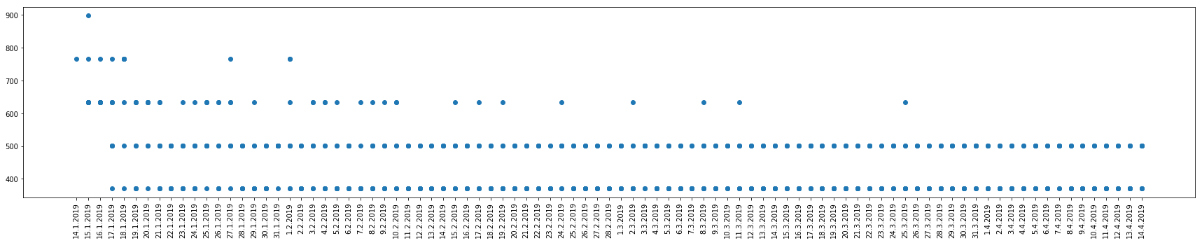
 This did not work out very well, there are too many values on the x axis.
Another way of visualizing the data:
fig = plt.figure(figsize=(30,5))
y = data_clean['Price']
x = data_clean['Departure Date']
plt.xticks(rotation=90)
plt.scatter(x, y)
plt.show()
This looks better, but it is still not very usable. We have to choose a more high-level approach.
How does the ticket price change throughout a day on average?
#Add new column classifyin the departure dates bz time
data_clean['Departure Time'].value_counts()
18:50    91
08:50    90
14:50    90
06:50    90
12:50    90
10:50    90
16:50    80
04:48    77
Name: Departure Time, dtype: int64
fig, (ax, ax2) = plt.subplots(ncols=2, figsize=[20, 6])
rep_plot = data_clean.groupby("Departure Time").mean().plot(kind='barh', title='Mean Price', legend=None, ax=ax).invert_yaxis()
rep_plot = data_clean.groupby("Departure Time").median().plot(kind='barh', title='Median Price', legend=None,ax=ax2).invert_yaxis()
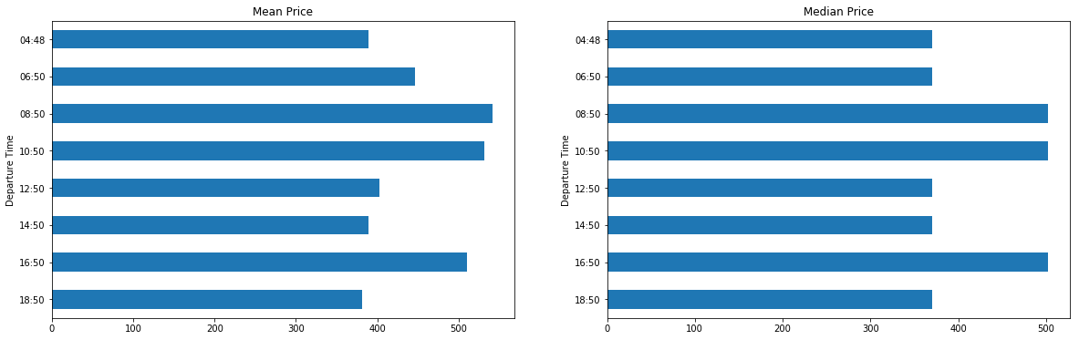
We can observe that the journeys at 08:50, 10:50, 16:50 are the most expensive. Better stay away from those times!
How does the ticket price change over a week?
pd.options.mode.chained_assignment = None # Disable warning
Add new column with departure date in datetime format:
data_clean['DepartureDate_dt'] = pd.to_datetime(data_clean['Departure Date'], format="%d.%m.%Y")
Create new column with the day of departure, based on the departure date:
data_clean['WeekDay'] = data_clean['DepartureDate_dt'].dt.day_name()
data_clean.head()
| Query Time | Departure Date | Departure Time | Arrival Date | Arrival Time | Price | DepartureDate_dt | WeekDay | |
|---|---|---|---|---|---|---|---|---|
| 0 | 14.01.2019 18:33:58 | 14.1.2019 | 18:50 | 14.1.2019 | 22:49 | 766 | 2019-01-14 | Monday |
| 1 | 14.01.2019 18:33:58 | 15.1.2019 | 04:48 | 15.1.2019 | 08:49 | 634 | 2019-01-15 | Tuesday |
| 2 | 14.01.2019 18:33:58 | 15.1.2019 | 06:50 | 15.1.2019 | 10:49 | 634 | 2019-01-15 | Tuesday |
| 3 | 14.01.2019 18:33:58 | 15.1.2019 | 08:50 | 15.1.2019 | 12:49 | 766 | 2019-01-15 | Tuesday |
| 4 | 14.01.2019 18:33:58 | 15.1.2019 | 10:50 | 15.1.2019 | 14:49 | 898 | 2019-01-15 | Tuesday |
cats = [ 'Monday', 'Tuesday', 'Wednesday', 'Thursday', 'Friday', 'Saturday', 'Sunday']
fig, (ax, ax2) = plt.subplots(ncols=2, figsize=[20, 6])
rep_plot = data_clean.groupby("WeekDay").median().reindex(cats).plot(kind='bar', legend=None, title='Median price over the week',ax=ax)
rep_plot = data_clean.groupby("WeekDay").mean().reindex(cats).plot(kind='bar', legend=None, title='Average price over the week', ax=ax2)
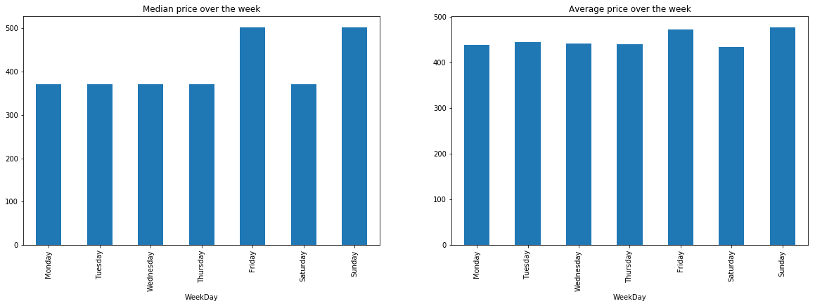
The most expensive journeys are on Fridays and Sundays, it might be because people are going to Vienna for the weekend on Friday or going to Vienna to work on Sunday.
Graphical summary
# @hidden_cell
fig, (ax, ax2) = plt.subplots(ncols=2, figsize=[20, 6])
rep_plot = data_clean.groupby("Departure Time").median().plot(kind='barh', title='Median Price', legend=None, ax=ax).invert_yaxis()
rep_plot = data_clean.groupby("Departure Time").mean().plot(kind='barh', title='Mean Price', legend=None,ax=ax2).invert_yaxis()
cats = [ 'Monday', 'Tuesday', 'Wednesday', 'Thursday', 'Friday', 'Saturday', 'Sunday']
fig, (ax, ax2) = plt.subplots(ncols=2, figsize=[20, 6])
rep_plot = data_clean.groupby("WeekDay").median().reindex(cats).plot(kind='bar', legend=None, title='Median price over the week',ax=ax)
rep_plot = data_clean.groupby("WeekDay").mean().reindex(cats).plot(kind='bar', legend=None, title='Average price over the week', ax=ax2)
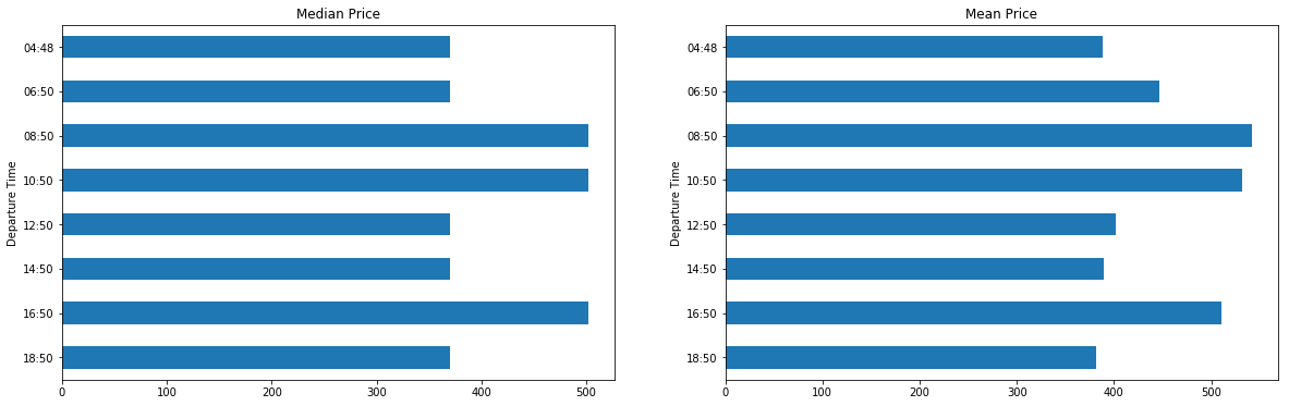
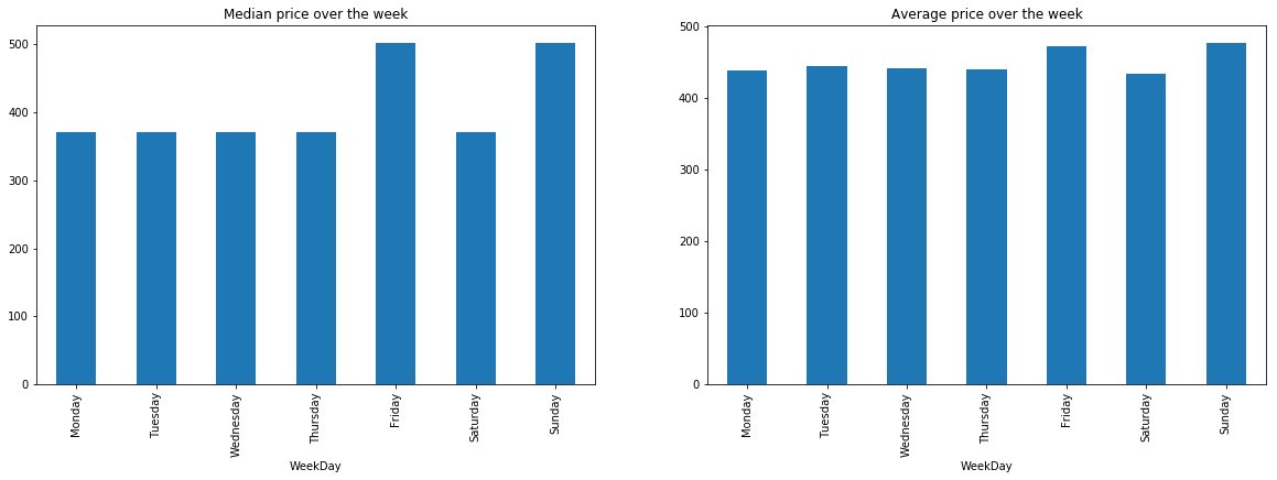
Do not travel on: Friday, Sunday
Do not travel at: 8:50, 12:50, 16:50