
Loan Default Prediction - University Project

Executive summary:
We are working with a dataset containing data related to US loans with deidentified periods. The dataset was provided in a coruse at NUS.
The aim of this notebook is to construct a model able to predict a loan default at a given time. That means we are not predicting whether the loan should be first handed out, but rather anticipating its default at a specific time snapshot.
A prediction at a certain time may serve as an input for calculating various risk metrics, such as exposure.
The dataset contains very few defaults, and therefore, we use oversampling to mitigate the problem of the model simply choosing the overrepresented class - non-defaulted loans. Several algorithms are tested and compared using confusion matrix as the principal evaluation tool.
%matplotlib inline
import pandas as pd
pd.set_option('display.max_columns', None)
pd.set_option('display.expand_frame_repr', False)
pd.set_option('max_colwidth', -1)
import numpy as np
import seaborn as sns
import matplotlib.pyplot as plt
from lifelines import KaplanMeierFitter
Data preprocessing
df = pd.read_pickle('loan_data.pkl')
df.head()
| Borrower | time | orig_time | first_time | mat_time | balance_time | LTV_time | interest_rate_time | hpi_time | uer_time | REtype_CO_orig_time | REtype_PU_orig_time | REtype_SF_orig_time | investor_orig_time | balance_orig_time | FICO_orig_time | Interest_Rate_orig_time | hpi_orig_time | default_time | payoff_time | status_time | |
|---|---|---|---|---|---|---|---|---|---|---|---|---|---|---|---|---|---|---|---|---|---|
| 0 | 1 | 25 | -7 | 25 | 113 | 41303.42 | 24.498336 | 9.2 | 226.29 | 4.7 | 0 | 0 | 1 | 0 | 45000.0 | 715 | 9.2 | 87.03 | 0 | 0 | 0 |
| 1 | 1 | 26 | -7 | 25 | 113 | 41061.95 | 24.483867 | 9.2 | 225.10 | 4.7 | 0 | 0 | 1 | 0 | 45000.0 | 715 | 9.2 | 87.03 | 0 | 0 | 0 |
| 2 | 1 | 27 | -7 | 25 | 113 | 40804.42 | 24.626795 | 9.2 | 222.39 | 4.4 | 0 | 0 | 1 | 0 | 45000.0 | 715 | 9.2 | 87.03 | 0 | 0 | 0 |
| 3 | 1 | 28 | -7 | 25 | 113 | 40483.89 | 24.735883 | 9.2 | 219.67 | 4.6 | 0 | 0 | 1 | 0 | 45000.0 | 715 | 9.2 | 87.03 | 0 | 0 | 0 |
| 4 | 1 | 29 | -7 | 25 | 113 | 40367.06 | 24.925476 | 9.2 | 217.37 | 4.5 | 0 | 0 | 1 | 0 | 45000.0 | 715 | 9.2 | 87.03 | 0 | 0 | 0 |
The data was given to us for analysis in a class at NUS with only the following description and a description of the variables:
We will be using a loan data set from the United States. The periods has been deidentified. As in the real world, loans may originate before the start of the observation period (this is an issue where loans are transferred between banks and investors as in securitization). The loan observations may thus be censored as the loans mature or borrowers refinance. The dataset contains the following variables:
Description of variables available in the dataset
Borrower: unique ID for each borrower
time: Time stamp of observation
orig_time: Time stamp for origination
first_time: Time stamp for first observation
mat_time: Time stamp for maturity
balance_time: Outstanding balance at observation time
LTV_time: Loan-to-value ratio at observation time, in %
interest_rate_time: Interest rate at observation time, in %
hpi_time: House price index at observation time, base year = 100
uer_time: Unemployment rate at observation time, in %
REtype_CO_orig_time: Real estate type condominium = 1, otherwise = 0
REtype_PU_orig_time: Real estate type planned urban development = 1, otherwise = 0
REtype_SF_orig_time: Single-family home = 1, otherwise = 0
investor_orig_time: Investor borrower = 1, otherwise = 0
balance_orig_time: Outstanding balance at origination time
FICO_orig_time: FICO score at origination time, in %
Interest_Rate_orig_time: Interest rate at origination time, in %
hpi_orig_time: House price index at origination time, base year = 100
default_time: Default observation at observation time
payoff_time: Payoff observation at observation time
status_time: Default (1), payoff (2), and nondefault/nonpayoff (0) observation at observation time
Install, Import modules, and configure settings
#Convert binary variables to categorical type, so that the correlation func will ignore them, leave out default_time as int64, since it will be a target variable
df['Borrower'] = df.Borrower.astype('object')
df['REtype_CO_orig_time'] = df.REtype_CO_orig_time.astype('object')
df['REtype_PU_orig_time'] = df.REtype_PU_orig_time.astype('object')
df['REtype_SF_orig_time'] = df.REtype_SF_orig_time.astype('object')
df['investor_orig_time'] = df.investor_orig_time.astype('object')
df['payoff_time'] = df.payoff_time.astype('int64')
df['status_time'] = df.status_time.astype('int64')
#Check if we were successful in changing the datatypes
df.info()
<class 'pandas.core.frame.DataFrame'>
RangeIndex: 622489 entries, 0 to 622488
Data columns (total 21 columns):
Borrower                   622489 non-null object
time                       622489 non-null int64
orig_time                  622489 non-null int64
first_time                 622489 non-null int64
mat_time                   622489 non-null int64
balance_time               622489 non-null float64
LTV_time                   622219 non-null float64
interest_rate_time         622489 non-null float64
hpi_time                   622489 non-null float64
uer_time                   622489 non-null float64
REtype_CO_orig_time        622489 non-null object
REtype_PU_orig_time        622489 non-null object
REtype_SF_orig_time        622489 non-null object
investor_orig_time         622489 non-null object
balance_orig_time          622489 non-null float64
FICO_orig_time             622489 non-null int64
Interest_Rate_orig_time    622489 non-null float64
hpi_orig_time              622489 non-null float64
default_time               622489 non-null int64
payoff_time                622489 non-null int64
status_time                622489 non-null int64
dtypes: float64(8), int64(8), object(5)
memory usage: 99.7+ MB
#Check for NA values
print("Missing values:", df.isnull().sum().sum())
df.dropna(inplace=True)
print("Missing values after dropping them:", df.isnull().sum().sum())
Missing values: 270
Missing values after dropping them: 0
#Show duplicates
print("Duplicate values:", df.duplicated().sum())
print("Duplicate values after removing them:", df.drop_duplicates(inplace=True))
Duplicate values: 305
Duplicate values after removing them: None
Exploratory analysis
Before we start the exploratory analysis, we prepare a dataset containing only loans originating and defaulting in our dataset. We will use this dataset to construct survival plots later in this section.
#Choose borrowers originated in the period covered in our dataset
dfs1 = df[df['orig_time'] == df['first_time']].copy()
# Choose borrowers who defaulted in the period covered in our dataset
defaulted_borrowers = dfs1[dfs1['default_time'] == 1]['Borrower'].to_list()
#Intersection of the two conditions
dfs2 = dfs1[dfs1['Borrower'].isin(defaulted_borrowers)].copy()
# Create a column with the lifespan of each borrower
dfs2['Duration'] = dfs2.groupby('Borrower')['Borrower'].transform('size')
kmf = KaplanMeierFitter()
Target variable - Distribution of defaulted loans and non-defaulted loan
# Check how many default we have in the data set
sns.countplot(x='default_time', data=df)
<matplotlib.axes._subplots.AxesSubplot at 0x28680021c88>
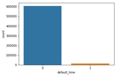
We observe that the dataset is heavily imbalanced. There are barely any defaults. To mitigate this issue, we will use an oversampling technique called SMOTE.
Number of unique borrowers
print('The number of unique borrowers is: ', len(df['Borrower'].unique()))
The number of unique borrowers is: 49982
Macroeconomic environment variables
plt.figure(figsize = (10, 15))
labels = ['House price index at origination time, base year = 100 ','House price index at observation time, base year = 100', 'Unemployment rate at observation time, in %']
# iterate through the new features
for i, feature in enumerate(['hpi_orig_time', 'hpi_time', 'uer_time']):
    # create a new subplot for each source
    plt.subplot(3, 1, i + 1)
    # plot repaid loans
    sns.kdeplot(df.loc[df['default_time'] == 0, feature], label = 'No default')
    # plot loans that were not repaid
    sns.kdeplot(df.loc[df['default_time'] == 1, feature], label = 'Default')

    # Label the plots
    plt.title(labels[i])
    plt.ylabel('Density');
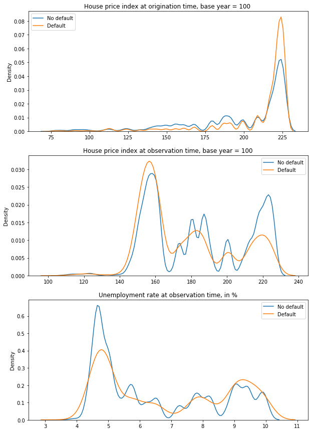
House price index at origination - the reason why defaulted loans show association with higher val real estate is expensive, people had to borrow more money to buy it, and therefore the loan carries more risk.
House price index at origination - one would expect the graph to be the opposite to what is shown, and therefore we have no theory related to the cause.
Unemployment rate at observation time - it seems that low unemployment rate at observation time is associated with loans not defaulting
Parameters of a loan at origination variables
plt.figure(figsize = (12, 30))
labels = ['Outstanding balance at origination time', 'Interest rate at origination time, in %']
# iterate through the new features
for i, feature in enumerate(['balance_orig_time', 'Interest_Rate_orig_time']):
    # create a new subplot for each source
    plt.subplot(4, 1, i + 1)
    # plot repaid loans
    sns.kdeplot(df.loc[df['default_time'] == 0, feature], label = 'No default')
    # plot loans that were not repaid
    sns.kdeplot(df.loc[df['default_time'] == 1, feature], label = 'Default')

    # Label the plots
    plt.title(labels[i])
    plt.xlabel('%s' % feature); plt.ylabel('Density');
binary_features = ['REtype_CO_orig_time', 'REtype_PU_orig_time', 'REtype_SF_orig_time']
T = dfs2["Duration"]
E = ~(dfs2["default_time"])
labels = ['Real estate type condominium', 'Real estate type planned urban development', 'Single-family home']

fig, axes = plt.subplots(len(binary_features), 1, figsize=(10, 20))
for i,feature in enumerate(binary_features):
    subset = (dfs2[feature] == 1)
    ax = plt.subplot(4,1,i+1)
    kmf.fit(T[subset], event_observed=E[subset], label=labels[i])
    kmf.plot(ax=ax)
    kmf.fit(T[~subset], event_observed=E[~subset], label="NOT " + labels[i])
    kmf.plot(ax=ax)
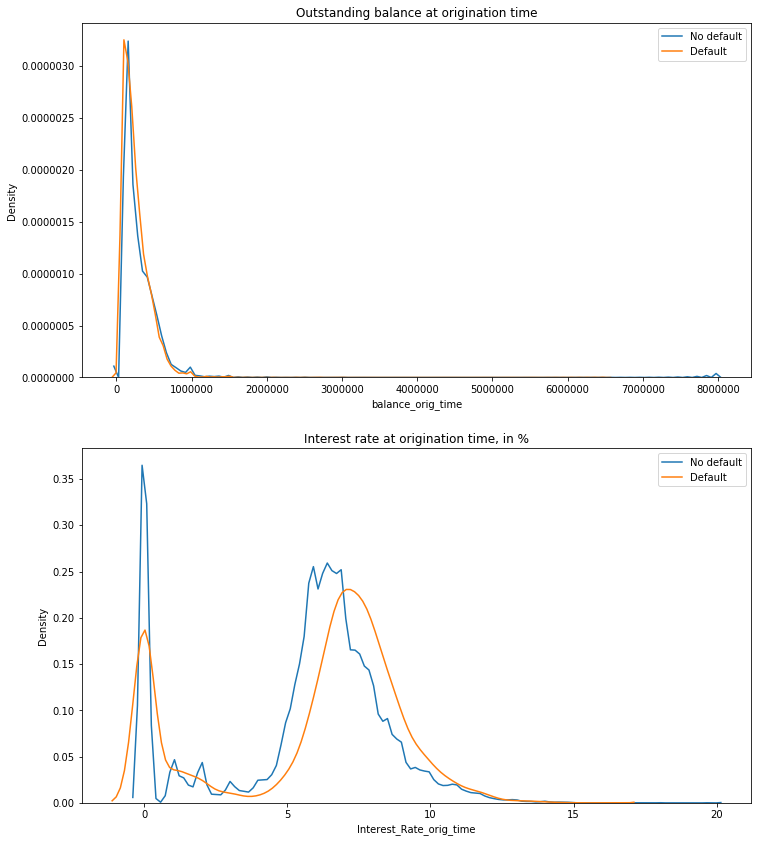
Interest rate at origination time - it seems that higher interest rate at origination time is associated with higher default risk. This is not surprising, since the interest should reflect the underlying risk.
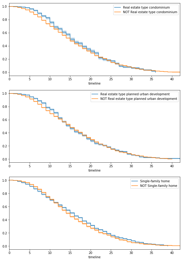
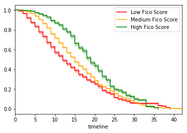
Survival plots - the three survival charts illustrate the relationship between the percentage of non-defaulted loans vs the observation time versus. The lower line is always the one for which less loans have “survived”
Variable parameters of a loan variables
plt.figure(figsize = (10, 10))
labels = ['Interest rate at observation time, in %', 'Outstanding balance at observation time', 'Loan-to-value ratio at observation time, in %']
variables = ['interest_rate_time', 'balance_time', 'LTV_time']
# iterate through the new features
for i, feature in enumerate(variables):
    # create a new subplot for each source
    plt.subplot(len(variables), 1, i + 1)
    # plot repaid loans
    sns.kdeplot(df.loc[df['default_time'] == 0, feature], label = 'No default')
    # plot loans that were not repaid
    sns.kdeplot(df.loc[df['default_time'] == 1, feature], label = 'Default')

    # Label the plots
    plt.title(labels[i])
    plt.xlabel('%s' % feature); plt.ylabel('Density');
plt.tight_layout()
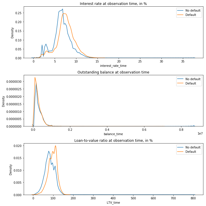
Interest rate at observation time - it seems that higher interest rate at observation time is associated with higher default risk. This is not surprising, since the interest should reflect the underlying risk.
Loan to value ratio at observation time - the higher the size of the loan relative to the value of the underlying asset, the higher the probablity of default. Borrower taking such loans are likely in financial need and more prone to default.
Borrower characteristics variables
#plt.figure(figsize = (10, 10))
labels = ['FICO score at origination time, in %']
variables = ['FICO_orig_time']
# iterate through the new features
for i, feature in enumerate(variables):
    # create a new subplot for each source
    plt.subplot(len(variables), 1, i + 1)
    # plot repaid loans
    sns.kdeplot(df.loc[df['default_time'] == 0, feature], label = 'No default')
    # plot loans that were not repaid
    sns.kdeplot(df.loc[df['default_time'] == 1, feature], label = 'Default')
    # Label the plots
    plt.title(labels[i])
    plt.xlabel('%s' % feature); plt.ylabel('Density');

fico_category = pd.cut(dfs2.FICO_orig_time,bins=[0,620,750, 850],labels=['Low Fico Score','Medium Fico Score','High Fico Score'])
if 'Fico Category' in dfs2.columns:
    dfs2.drop(columns=['Fico Category'], inplace=True)
dfs2.insert(16,'Fico Category',fico_category)
fico_categories = ['Low Fico Score','Medium Fico Score','High Fico Score']
colors = ['red', 'orange', 'green']
ax = plt.subplot(1,1,1)
for i, cat in enumerate(fico_categories):
    kmf.fit(dfs2[dfs2['Fico Category'] == cat]['Duration'], ~dfs2[dfs2['Fico Category'] == cat]['default_time'])
    kmf.plot(ax=ax, label=cat, c=colors[i])
binary_features = ['investor_orig_time']
T = dfs2["Duration"]
E = ~(dfs2["default_time"])
labels = ['Investor borrower']
fig, axes = plt.subplots(len(binary_features), 1, figsize=(10, 20))
for i,feature in enumerate(binary_features):
    subset = (dfs2[feature] == 1)
    ax = plt.subplot(4,1,i+1)
    kmf.fit(T[subset], event_observed=E[subset], label=labels[i])
    kmf.plot(ax=ax)
    kmf.fit(T[~subset], event_observed=E[~subset], label="NOT " + labels[i])
    kmf.plot(ax=ax)

Fico score at observation time - Loans with higher FICO score are less likely to default. Expected observation since FICO score is a credit rating score.
Distribution plots for all variables
# Check the data distributions for every column
df.hist(bins=30, figsize=(30,20))
plt.show()
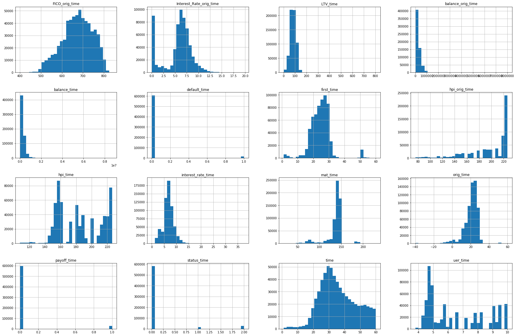
For some histograms, we see large unused spaces on the x axis. That signifies the presence of outliers. We will explore LTV_time, balance_orig_time, balance_time, interest_rate_time
Boxplots for all continuous variables
df.select_dtypes(exclude=['object']).columns.tolist()
['time',
 'orig_time',
 'first_time',
 'mat_time',
 'balance_time',
 'LTV_time',
 'interest_rate_time',
 'hpi_time',
 'uer_time',
 'balance_orig_time',
 'FICO_orig_time',
 'Interest_Rate_orig_time',
 'hpi_orig_time',
 'default_time',
 'payoff_time',
 'status_time']
# Economic environment features
plt.figure(figsize = (15, 20))
# iterate through the new features
for i, column in enumerate(df.select_dtypes(exclude=['object']).columns.tolist()):
    # create a new subplot for each source, subplot(number of rows, number of columns, id of subplot)
    plt.subplot(8, 2, i+1)
    sns.boxplot(data=df, x=column)
plt.tight_layout()
The section below was used to manually remove outliers. However, when I tested the models with the outliers unremoved, it performed better. It might be due to the fact that I use the sklearn scaler or that the outliers were removed in a wrong way. In sum, I left the outliers untouched and commented out the code for manually removing them.
#Remove outliers to achieve a more normal distributions
dfc = df.copy()
# dfc = df[df['balance_time'] < 6000000]
# dfc = dfc[dfc['LTV_time'] < 500]
# dfc = dfc[dfc['interest_rate_time'] < 20]
# dfc = dfc[dfc['balance_orig_time'] < 6000000]
# dfc = dfc[dfc['Interest_Rate_orig_time'] < 20]
Variable selection
#Check how the defaulted rows look like
dfc[dfc['default_time'] == 1].head()
| Borrower | time | orig_time | first_time | mat_time | balance_time | LTV_time | interest_rate_time | hpi_time | uer_time | REtype_CO_orig_time | REtype_PU_orig_time | REtype_SF_orig_time | investor_orig_time | balance_orig_time | FICO_orig_time | Interest_Rate_orig_time | hpi_orig_time | default_time | payoff_time | status_time | |
|---|---|---|---|---|---|---|---|---|---|---|---|---|---|---|---|---|---|---|---|---|---|
| 23 | 1 | 48 | -7 | 25 | 113 | 29087.21 | 26.658065 | 9.200 | 146.45 | 8.3 | 0 | 0 | 1 | 0 | 45000.0 | 715 | 9.20 | 87.03 | 1 | 0 | 1 |
| 99 | 6 | 56 | 19 | 25 | 139 | 190474.11 | 75.834755 | 6.580 | 181.43 | 6.6 | 0 | 0 | 1 | 0 | 212000.0 | 670 | 6.58 | 191.42 | 1 | 0 | 1 |
| 115 | 9 | 37 | 18 | 25 | 138 | 130140.31 | 99.138105 | 8.000 | 153.35 | 9.0 | 0 | 0 | 1 | 0 | 128000.0 | 501 | 8.00 | 186.91 | 1 | 0 | 1 |
| 120 | 10 | 29 | 18 | 25 | 139 | 88046.35 | 67.296390 | 10.230 | 217.37 | 4.5 | 0 | 0 | 1 | 0 | 90000.0 | 665 | 7.20 | 186.91 | 1 | 0 | 1 |
| 146 | 16 | 34 | 18 | 25 | 138 | 160044.34 | 73.431289 | 9.875 | 173.35 | 5.8 | 0 | 0 | 1 | 0 | 164500.0 | 572 | 7.50 | 186.91 | 1 | 0 | 1 |
Correlation matrix
corr_matrix = dfc.corr()
mask = np.zeros_like(corr_matrix, dtype=np.bool)
mask[np.triu_indices_from(mask)]= True
f, ax = plt.subplots(figsize=(20, 25))
heatmap = sns.heatmap(corr_matrix,
                      mask = mask,
                      square = True,
                      linewidths = .5,
                      cmap = 'coolwarm',
                      cbar_kws = {'shrink': .4,
                                'ticks' : [-1, -.5, 0, 0.5, 1]},
                      vmin = -1,
                      vmax = 1,
                      annot = True,
                      annot_kws = {'size': 12})
#add the column names as labels
ax.set_yticklabels(corr_matrix.columns, rotation = 0)
ax.set_xticklabels(corr_matrix.columns)
ax.tick_params(labelsize=15)
sns.set_style({'xtick.bottom': True}, {'ytick.left': True})
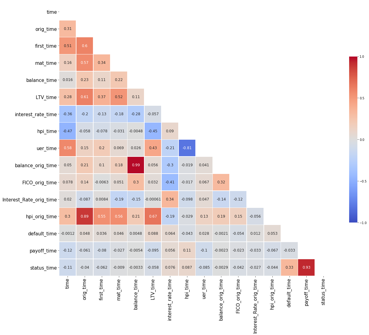
We see no perfect correlation, therefore, we do not need to drop any variables.
Define predictors
Basic predictor selection based on common sense
#Subset a data not to include the last three columns. Those columns are default_time, payoff_time, status_time.
#They are related to the target variable, and therefore we dont want them in our X variable
X = dfc[dfc.columns[1:-3]]
dfc.columns[1:-3]
Index(['time', 'orig_time', 'first_time', 'mat_time', 'balance_time',
       'LTV_time', 'interest_rate_time', 'hpi_time', 'uer_time',
       'REtype_CO_orig_time', 'REtype_PU_orig_time', 'REtype_SF_orig_time',
       'investor_orig_time', 'balance_orig_time', 'FICO_orig_time',
       'Interest_Rate_orig_time', 'hpi_orig_time'],
      dtype='object')
Define target variable
y = dfc['default_time']
Variable selection through correlation
The idea is to see which independent variables are strong correlated with the target variable. In this case, the threshold is 0.5. It yields only the target variable itself. Therefore, we must use another method.
#Selecting highly correlated features
high_corr_features = corr_matrix[(abs(corr_matrix) > 0.8) & (corr_matrix != 1)]
high_corr_features = high_corr_features.dropna(axis=1, how='all')
high_corr_features
| orig_time | balance_time | hpi_time | uer_time | balance_orig_time | hpi_orig_time | payoff_time | status_time | |
|---|---|---|---|---|---|---|---|---|
| time | NaN | NaN | NaN | NaN | NaN | NaN | NaN | NaN |
| orig_time | NaN | NaN | NaN | NaN | NaN | 0.886296 | NaN | NaN |
| first_time | NaN | NaN | NaN | NaN | NaN | NaN | NaN | NaN |
| mat_time | NaN | NaN | NaN | NaN | NaN | NaN | NaN | NaN |
| balance_time | NaN | NaN | NaN | NaN | 0.985177 | NaN | NaN | NaN |
| LTV_time | NaN | NaN | NaN | NaN | NaN | NaN | NaN | NaN |
| interest_rate_time | NaN | NaN | NaN | NaN | NaN | NaN | NaN | NaN |
| hpi_time | NaN | NaN | NaN | -0.811461 | NaN | NaN | NaN | NaN |
| uer_time | NaN | NaN | -0.811461 | NaN | NaN | NaN | NaN | NaN |
| balance_orig_time | NaN | 0.985177 | NaN | NaN | NaN | NaN | NaN | NaN |
| FICO_orig_time | NaN | NaN | NaN | NaN | NaN | NaN | NaN | NaN |
| Interest_Rate_orig_time | NaN | NaN | NaN | NaN | NaN | NaN | NaN | NaN |
| hpi_orig_time | 0.886296 | NaN | NaN | NaN | NaN | NaN | NaN | NaN |
| default_time | NaN | NaN | NaN | NaN | NaN | NaN | NaN | NaN |
| payoff_time | NaN | NaN | NaN | NaN | NaN | NaN | NaN | 0.932983 |
| status_time | NaN | NaN | NaN | NaN | NaN | NaN | 0.932983 | NaN |
Lets drop orig_time, balance_time, hpi_time because of high multicolinearity.
# drop by Name
X = X.drop(['orig_time', 'balance_time', 'hpi_time'], axis=1)
Variable selection through Feature Importance
Bagged decision trees like Random Forest and Extra Trees can be used to estimate the importance of features.
I fit a random forest on the data, then created a DataFrame with the improtances and the features and selected only features
with importance higher than 0.05. (arbitrary threshold which cuts out the binary variables who naturally have a lowee variance)
Source: https://machinelearningmastery.com/feature-selection-machine-learning-python/
from sklearn.ensemble import ExtraTreesClassifier
# load data
# feature extraction
model = ExtraTreesClassifier(n_estimators=10)
model.fit(X, y)
print(model.feature_importances_)
[0.08349057 0.0623258  0.07059034 0.16763307 0.1205299  0.05678918
 0.00491261 0.00596746 0.01155812 0.00612766 0.13021501 0.12694113
 0.09385999 0.05905915]
dictionary = dict(zip(model.feature_importances_.tolist(), X.columns))
importance = pd.DataFrame(list(dictionary.items()), columns=['Importance', 'Feature'])
importance.sort_values(by='Importance', ascending=False)
| Importance | Feature | |
|---|---|---|
| 3 | 0.167633 | LTV_time |
| 10 | 0.130215 | balance_orig_time |
| 11 | 0.126941 | FICO_orig_time |
| 4 | 0.120530 | interest_rate_time |
| 12 | 0.093860 | Interest_Rate_orig_time |
| 0 | 0.083491 | time |
| 2 | 0.070590 | mat_time |
| 1 | 0.062326 | first_time |
| 13 | 0.059059 | hpi_orig_time |
| 5 | 0.056789 | uer_time |
| 8 | 0.011558 | REtype_SF_orig_time |
| 9 | 0.006128 | investor_orig_time |
| 7 | 0.005967 | REtype_PU_orig_time |
| 6 | 0.004913 | REtype_CO_orig_time |
# drop by Name
X = X.drop(['REtype_SF_orig_time', 'investor_orig_time', 'REtype_PU_orig_time', 'REtype_CO_orig_time'], axis=1)
Create test/train split
from sklearn.model_selection import train_test_split
X_train_raw, X_test_raw, y_train, y_test = train_test_split(X, y.values, test_size=0.3, random_state=0)
Normalize data
Some ML algorithms such as SVM require scaling, logistic regression, decision trees, and random forests do not
from sklearn.preprocessing import StandardScaler

stdsc = StandardScaler()
X_train = stdsc.fit_transform(X_train_raw)
X_test = stdsc.transform(X_test_raw)
Define functions for model fitting, prediction and evaluation
from sklearn.linear_model import LogisticRegression
from sklearn.ensemble import RandomForestClassifier
from sklearn.tree import DecisionTreeClassifier
import xgboost as xgb
from sklearn.svm import SVC
from sklearn.neighbors import KNeighborsClassifier
from sklearn.neural_network import MLPClassifier
Create a dictionary with sklearn algorithms to be used
different_model_comparison = {
    "Random Forest":RandomForestClassifier(random_state=0,n_estimators=10),
    "Logistic Regression":LogisticRegression(random_state=0,  solver='lbfgs'),
    "Decision Tree":DecisionTreeClassifier(random_state=0),
    "XGBoost":xgb.XGBClassifier(objective="binary:logistic", random_state=42),
    "MLP":MLPClassifier(solver='lbfgs', alpha=1e-5, hidden_layer_sizes=(5, 2), random_state=1)
     #"SVM":SVC(random_state=0,probability=True) #too slow never finished
}
Component 1: Model fitting function
# function to train models, return a dictionary of trained models
# Input is the dictionary with ML models, we use the functions so that we can train more models at once
def train_model(model_dict,X_train,y_train):
    for model in model_dict:
        print("Training:",model)
        model_dict[model].fit(X_train,y_train)
    return model_dict
Component 2: Model evaluation function
# Wrapping this function so we can easily change the model and evaluate them
# function to evaluate model performance
from sklearn import metrics
def model_eval(clf_name,clf,X_test,y_test):
    print("Evaluating:",clf_name)
    y_pred = clf.predict(X_test)
    y_score = clf.predict_proba(X_test)[:,1]
    confusion_matrix = metrics.confusion_matrix(y_test, y_pred)
    report = pd.Series({
        "model":clf_name,
        "precision":metrics.precision_score(y_test, y_pred),
        "recall":metrics.recall_score(y_test, y_pred),
        "accuracy score":metrics.accuracy_score(y_test, y_pred),
        'roc_auc_score' : metrics.roc_auc_score(y_test, y_score)
    })
    return report,confusion_matrix
Parent model fitting and evaluation function
def train_eval_model(model_dict,X_train,y_train,X_test,y_test):
    cols = ['model', 'roc_auc_score', 'precision', 'recall', 'accuracy score']
    model_report = pd.DataFrame(columns = cols)
    confusion_matrix_dict = {}
    model_dict = train_model(model_dict,X_train,y_train)
    for model in model_dict:
        report,confusion_matrix = model_eval(model,model_dict[model],X_test,y_test)
        model_report = model_report.append(report,ignore_index=True)
        confusion_matrix_dict[model] = confusion_matrix
        #confusion matrix
        plt.figure(figsize=(3,3))
        plt.title(model)
        sns.heatmap(pd.DataFrame(confusion_matrix), annot=True, cmap="YlGnBu" ,fmt='g')
        plt.xlabel('Model Prediction')
        plt.ylabel('Actual loan status')
    return model_report,confusion_matrix_dict
Action! Model training and evaluating
Train and evaluate model: Approach as covered in class
model_report,confusion_matrix_dict = train_eval_model(different_model_comparison,X_train,y_train,X_test,y_test)
Training: Random Forest
Training: Logistic Regression
Training: Decision Tree
Training: XGBoost
Training: MLP
Evaluating: Random Forest
Evaluating: Logistic Regression
Evaluating: Decision Tree
Evaluating: XGBoost


C:\Users\Martin\Anaconda3\lib\site-packages\sklearn\metrics\classification.py:1437: UndefinedMetricWarning: Precision is ill-defined and being set to 0.0 due to no predicted samples.
  'precision', 'predicted', average, warn_for)


Evaluating: MLP


C:\Users\Martin\Anaconda3\lib\site-packages\sklearn\metrics\classification.py:1437: UndefinedMetricWarning: Precision is ill-defined and being set to 0.0 due to no predicted samples.
  'precision', 'predicted', average, warn_for)
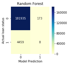
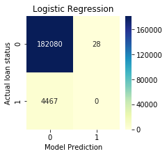
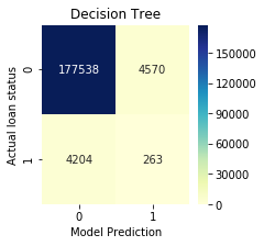
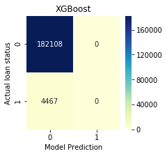
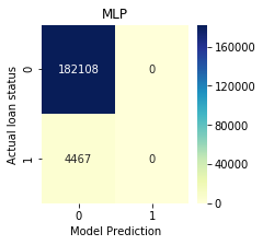
#Models above poor, since they cannot predict loan defaults well
print("Defaulted loans in the dataset:", y_test[y_test == 1].shape[0])
Defaulted loans in the dataset: 4467
Every model, except for decision tree, was unable to predict ANY of the defaulted loans! Let us try the oversampling approach then.
Train and evaluate model: Oversampling approach
from imblearn.over_sampling import SMOTE

X_train_bal, y_train_bal = SMOTE(random_state=0).fit_sample(X_train,y_train)
X_test_bal, y_test_bal = X_test, y_test
#Compare train dataset used before and now. Now, the dataset is balanced in respect to default/non-default
print("Share of defaulted loans in the original training dataset", sum(y_train)/len(y_train))
print("Share of defaulted loans in the oversampled training dataset", sum(y_train_bal)/len(y_train_bal))
Share of defaulted loans in the original dataset 0.024539496805937443
Share of defaulted loans in the oversampled dataset 0.5
model_report_bal,cm_dict_bal = train_eval_model(different_model_comparison,X_train_bal,y_train_bal,X_test_bal,y_test_bal)
Training: Random Forest
Training: Logistic Regression
Training: Decision Tree
Training: XGBoost
Training: MLP
Evaluating: Random Forest
Evaluating: Logistic Regression
Evaluating: Decision Tree
Evaluating: XGBoost
Evaluating: MLP
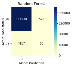
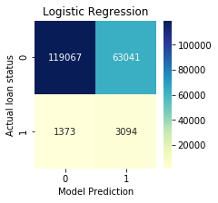
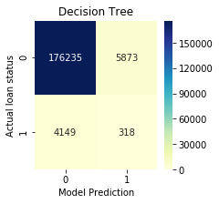
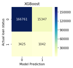
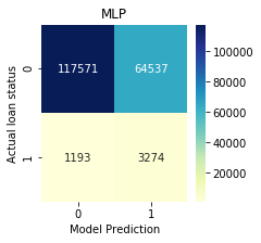
print("Defaulted loans in the dataset:", y_test_bal[y_test_bal == 1].shape[0])
Defaulted loans in the dataset: 4467
Unlike with the imbalanced training dataset, we can see that no model has failed with predicting all of the 4467 defaults in the test dataset.
Model commentary
The variant using balanced training data is much better at predicting defaults. However, the downside is that we have a higher number of loans for which we wrongly predict failure. In this model working with the observation period, it would mean that the instituition holding the loans would likely unnecessarily hedge itself against the expected failure.
If the model was predicting default only from the origination data, it would mean that we would lose money, since we would not be giving loans to subjects who would be able to pay them.
In order to carry out a proper assessment of the model, it would be necessary to define custom functions calculating the cost of not accepting a loan application versus having a borrower default.
Compare the approaches above
model_report
| model | roc_auc_score | precision | recall | accuracy score | |
|---|---|---|---|---|---|
| 0 | Random Forest | 0.608173 | 0.044199 | 0.001791 | 0.975174 |
| 1 | Logistic Regression | 0.726111 | 0.000000 | 0.000000 | 0.975908 |
| 2 | Decision Tree | 0.516891 | 0.054418 | 0.058876 | 0.952973 |
| 3 | XGBoost | 0.758559 | 0.000000 | 0.000000 | 0.976058 |
| 4 | MLP | 0.750362 | 0.000000 | 0.000000 | 0.976058 |
model_report_bal
| model | roc_auc_score | precision | recall | accuracy score | |
|---|---|---|---|---|---|
| 0 | Random Forest | 0.627585 | 0.079618 | 0.011193 | 0.973228 |
| 1 | Logistic Regression | 0.728628 | 0.046783 | 0.692635 | 0.654755 |
| 2 | Decision Tree | 0.519469 | 0.051365 | 0.071189 | 0.946284 |
| 3 | XGBoost | 0.723225 | 0.063579 | 0.233266 | 0.899386 |
| 4 | MLP | 0.755964 | 0.048281 | 0.732930 | 0.647702 |
Comparing the training imbalanced and balanced dataset, we see a marked improvement in recall, which is a metric fitting for our usecase, as opposed to accuracy. We are using recall as an evaluation metric, since we believe that a defaulted loan has a severe impact on the creditor.
In reality, we would likely select logistic regression to be used in production, since it offers good predictions coupled with much easier interpretability than the second-best algorithm MLP.
Sources:
1) Code - https://github.com/XC-Li/Loan_Default_Prediction
2) Code - https://github.com/lucastravi/mortgage_backed_securities/blob/master/mortgage_back_securities.ipynb
3) Theory - https://beckernick.github.io/oversampling-modeling/
5) Precision/Recall - https://hackernoon.com/idiots-guide-to-precision-recall-and-confusion-matrix-b32d36463556
6) Survival Analysis - https://lifelines.readthedocs.io/en/latest/