
What influences hotel prices in Singapore?

Executive summary
This article documents the process of building a simple regression model to show the association between information regarding a hotel available on Booking.com and the price of a hotel room. There are several challenges and limitations related to the modelling which are described at the end of the article in a greater detail.
Import necessary libraries
import pandas as pd
import matplotlib.pyplot as plt
import seaborn as sns
import numpy as np
from scipy import stats
import numpy as np
import statsmodels.api as sm
import seaborn as sns
from matplotlib import pyplot as plt
import matplotlib.style as style
import matplotlib.gridspec as gridspec
%matplotlib inline
Import data
The data was scraped from Booking.com using Octoparse. The scraping was carried out on November 8, 2019 for three nights of stay - Dec 20, 2019 to Dec 22 2019. The prices are the sum of the price for the cheapest room at the hotel available at Booking.com (the prices that are shown when searching for accomodation)for the two nights, if there is a Christmas holiday effect, we assume it acts on all the hotels in the same way.
Below is the url for the search.
https://www.booking.com/searchresults.html?aid=304142&label=gen173nr-1DCAEoggI46AdIM1gEaMkBiAEBmAExuAEXyAEM2AED6AEB-AECiAIBqAIDuAK27o_uBcACAQ&sid=9ea3a2ea7e79bbd28734b6438faaece0&tmpl=searchresults&checkin_month=12&checkin_monthday=20&checkin_year=2019&checkout_month=12&checkout_monthday=22&checkout_year=2019&city=-73635&class_interval=1&dest_id=-73635&dest_type=city&from_sf=1&group_adults=2&group_children=0&label_click=undef&no_rooms=1&raw_dest_type=city&room1=A%2CA&sb_price_type=total&shw_aparth=0&slp_r_match=0&src=searchresults&srpvid=c84b709ef1cf01ad&ss=Singapore&ssb=empty&ssne=Singapore&ssne_untouched=Singapore&top_ufis=1&nflt=ht_id%3D204%3Boos%3D1%3B&rsf=
url = 'https://raw.githubusercontent.com/MartinMaka/martinmaka.github.io/master/assets/datsets/sg_hotels.csv'
df = pd.read_csv(url, decimal=".")
df.drop(columns=['Distance from centre in metres'], inplace=True)
df.head()
| Name | Distance from Changi Airport in km | Hotel Stars | District | Number of Reviews | Guest Rating | Price in SGD | Extra Fees | Final Price | Subway Access | Love Hotel | |
|---|---|---|---|---|---|---|---|---|---|---|---|
| 0 | Hotel Boss | 14.7 | 4 | Kallang | 14,096 | 7.5 | 263 | 47 | 310 | 1 | 0 |
| 1 | Crowne Plaza Changi Airport | 0.5 | 5 | Changi | 5,375 | 9.0 | 495 | 88 | 583 | 1 | 0 |
| 2 | Hotel Bencoolen Singapore | 16.0 | 3 | Bencoolen | 552 | 7.0 | 255 | 45 | 300 | 1 | 0 |
| 3 | Marina Bay Sands | 15.6 | 5 | Marina Bay | 30,828 | 8.9 | 1038 | 184 | 1222 | 1 | 0 |
| 4 | Shangri-La Hotel Singapore | 18.1 | 5 | Orchard | 2,436 | 9.1 | 512 | 91 | 603 | 0 | 0 |
df.info()
<class 'pandas.core.frame.DataFrame'>
RangeIndex: 299 entries, 0 to 298
Data columns (total 11 columns):
Name                                  299 non-null object
Distance from Changi Airport in km    299 non-null float64
Hotel Stars                           299 non-null int64
District                              299 non-null object
Number of Reviews                     299 non-null object
Guest Rating                          299 non-null float64
Price in SGD                          299 non-null int64
Extra Fees                            299 non-null int64
Final Price                           299 non-null int64
Subway Access                         299 non-null int64
Love Hotel                            299 non-null int64
dtypes: float64(2), int64(6), object(3)
memory usage: 25.8+ KB
Discussion of data types assigned to columns
‘Hotel Stars’ - an integer, but this value is actually categorical. We have to convert it to dummies later.
‘Number of Reviews’ - an object, but the value is numerical. We need to convert it to an integer.
‘Guest Rating’ - a float, but we might be tempted to convert it into a categorical variable if there is a limited number of unique values. However, the ratings are on an ordinal scale, and therefore, we can leave them as floats.
‘Subway Access’ and ‘Love Hotel’ - these variables are integers, but they are actually binary variables. We need to convert them.
df['Hotel Stars'] = df['Hotel Stars'].astype(object)

df['Number of Reviews'] = df['Number of Reviews'].apply(lambda x: str(x.replace(',','')))
df['Number of Reviews'] = df['Number of Reviews'].astype(int)

df['Subway Access'] = df['Subway Access'].astype(int)
df['Love Hotel'] = df['Love Hotel'].astype(int)
Exploratory data analysis
Description of the variables in the dataset and their expected impact on the final price
- Name
This is just a name of the hotel. It might happen that the most famous hotel in Singapore, Marina Bay Sands, will be significantly more expensive than others. However, we do not want to use this variable as a predictor and therefore we will not use it in our analysis. - Distance from Changi Airport in km
How far the hotel is from the Singapore Airport. We expect that hotels close to the airport should be more expensive than the ones far from the airport. - Hotel Stars
We expect that hotels with more stars will be more expensive than hotels with low stars. - District
The district the hotel is located in. The expectation is that more attractive districts will harbour more expensive hotels. - Distance from centre in metres
The expectation is that the closer the hotel is to the city centre, the more expensive it will be. - Number of Reviews
Hotels with more reviews will probably be more expensive, since they possess something special the customers want to share. On the other hand, a negative experience could also result in a high review number. - Guest Rating
We expect that the higher the guest rating, the more expensive the hotel. This variable is likely going to capture factors not included in the other variables. Additionally, it might also be highly correlated with some other independent variables. - Price in SGD
Base price of the cheapest room in the hotel. - Extra Fees
Extra fees on top of the base price. As of February 2020, Booking.com does not show this item. - Final Price
Target variable. A sum of the base price and the extra fees. - Subway Access
We expect that hotels with a subway access will be more expensive than the ones without it. - Love Hotel
Hotels that provide rooms with hourly rates. These hotels come from two chains - ‘Hotel 81’ and ‘Fragrance Hotel’ We expect these hotels to be less expensive than other hotels.
Distance from Changi Airport
# Plot
plt.figure(figsize=(7.5,5))
sns.scatterplot(y=df['Final Price'], x=df['Distance from Changi Airport in km']);
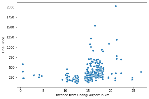
We can see that there are actually clusters based on the distance from the airport and quite a few outliers. We will can try to arbitrarily cluster the data into three distinct groups - close, middle, and far.
df['airport_distance'] = pd.cut(df['Distance from Changi Airport in km'], bins=[0, 8, 20, 200], labels=['close','middle','far'])
sns.boxplot(df['airport_distance'], df['Final Price']);
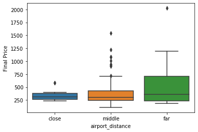
The boxplots show that the further away the hotel is from the airport, the higher the price. However, the hotels far away might also possess other chaarcteristics that make them expensive and the distance is not the primary price driver.
Hotel Stars
sns.boxplot(df['Hotel Stars'], df['Final Price'])
<matplotlib.axes._subplots.AxesSubplot at 0x7f4c9a4bc160>
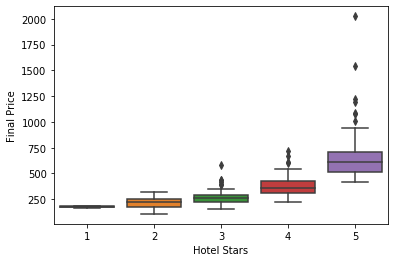
As expected, the more stars the hotel has, the higher the final price. We can also observe that as the stars increase, the more outliers appear. This likely has to do with the fact that the four-star and five-star hotels differentiate themselves much more than hotels with less than four stars.
Again, we can group the values. Hotels with one to three stars seem similar in terms of their price.
df['hotel_star_category'] = pd.cut(df['Hotel Stars'], bins=[0, 3, 4, 5], labels=['low-class','four_star','five_star'])
sns.boxplot(df['hotel_star_category'], df['Final Price']);

District
len(df['District'].unique())
34
plt.figure(figsize=(10,4))
ax =df['District'].value_counts().plot(kind='bar')
ax.set_xticklabels(ax.get_xticklabels(), rotation=40, ha="right")
plt.axhline(10, color='r')
plt.tight_layout()

We have 34 different districts, but the majority of the districts have less than 10 hotels located in them.
from numpy import mean
district_mean_price = df.groupby(['District'])['Final Price'].mean().reset_index().sort_values(by='Final Price', ascending=False)
plt.figure(figsize=(20,4))
ax= sns.barplot(district_mean_price['District'], district_mean_price['Final Price'])
ax.set_xticklabels(ax.get_xticklabels(), rotation=40, ha="right")
plt.axhline(district_mean_price['Final Price'].mean(), color='r')
plt.tight_layout()
plt.show()

There are large price differences in the mean price of hotels per district. However, we have to keep in mind that most of the districts have less than 10 hotels located in them, and therefore the mean prices might be skewed by outliers. We will not use districts in the analysis, since there is too many of them. The most expensive district ‘Sentosa Island’ definitely contains an outlier as seen below:
df[df['District'] == 'Sentosa Island'][['Name','Final Price']]
| Name | Final Price | |
|---|---|---|
| 43 | The Outpost Hotel Sentosa by Far East Hospitality | 784 |
| 76 | Village Hotel Sentosa by Far East Hospitality | 720 |
| 126 | Le Méridien Singapore, Sentosa | 1192 |
| 192 | W Singapore - Sentosa Cove | 1088 |
| 194 | Capella Singapore | 2024 |
Number of Reviews
plt.figure(figsize=(7.5,5))
sns.scatterplot(y=df['Final Price'], x=df['Number of Reviews']);
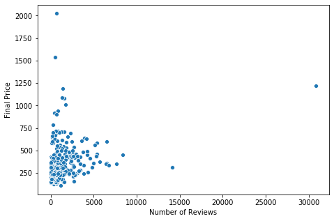
The scatterplot shows two extreme outliers in terms of the number of guestreviews. Let us see what hotels those are and produce a scatterplot without them.
df[df['Number of Reviews'] > 10000][['Name','Number of Reviews']]
| Name | Number of Reviews | |
|---|---|---|
| 0 | Hotel Boss | 14096 |
| 3 | Marina Bay Sands | 30828 |
Marina Bay Sands, the hallmark of Singapore, is unsurprisingly at the top of the list.
plt.figure(figsize=(7.5,5))
ax = sns.scatterplot(y=df[df['Number of Reviews'] < 10000]['Final Price'], x=df[df['Number of Reviews'] < 10000]['Number of Reviews']);
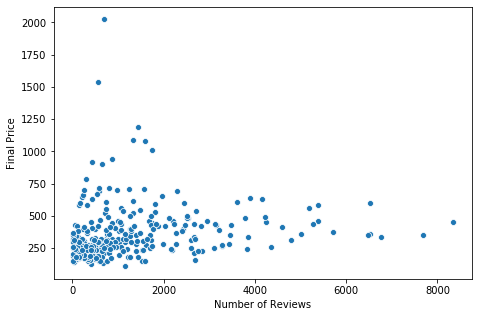
If we look at the scatterplot without the two outliers, we see no clear relationship between the number of hotel reviews and the hotel price. This variable might not be a good predictor.
Guest Rating
sns.scatterplot(y=df['Final Price'], x=df['Guest Rating']);
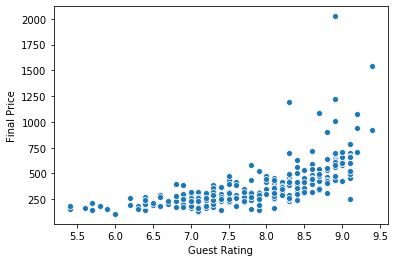
We see a roughly linear relationship between the guest rating and the final price. Based on this graph, guest rating is very likely going to exhibit the strongest association with the final price out of all the independent variables.
Subway Access
sns.boxplot(y=df['Final Price'], x=df['Subway Access']);
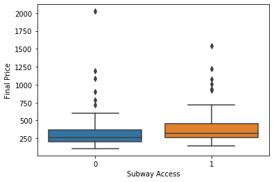
We see that there is a small difference in the price between hotels with a subway access and those without it. We are not going to use this predictor.
Love Hotel
sns.boxplot(y=df['Final Price'], x=df['Love Hotel']);
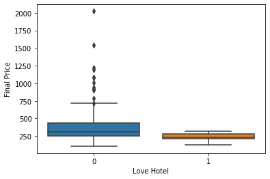
It seems that there is a difference in the prices for love hotels and normal hotels, let see later if it could be a good independent variable.
Target variable
Let us plot the distribution of the target variable
    ## Creating a customized chart. and giving in figsize and everything.
    fig = plt.figure(constrained_layout=True, figsize=(15,5))
    ## creating a grid of 3 cols and 3 rows.
    grid = gridspec.GridSpec(ncols=3, nrows=1, figure=fig)
    #gs = fig3.add_gridspec(3, 3)

    ## Customizing the histogram grid.
    ax1 = fig.add_subplot(131)
    ## Set the title.
    ax1.set_title('Histogram')
    ## plot the histogram.
    sns.distplot(df.loc[:,'Final Price'], norm_hist=True, ax = ax1)

    # customizing the QQ_plot.
    ax2 = fig.add_subplot(132)
    ## Set the title.
    ax2.set_title('QQ_plot')
    ## Plotting the QQ_Plot.
    stats.probplot(df.loc[:,'Final Price'], plot = ax2)

    ## Customizing the Box Plot.
    ax3 = fig.add_subplot(133)
    ## Set title.
    ax3.set_title('Box Plot')
    ## Plotting the box plot.
    sns.boxplot(df.loc[:,'Final Price'], orient='v', ax = ax3 );
plt.tight_layout()

    ## Creating a customized chart. and giving in figsize and everything.
    fig = plt.figure(constrained_layout=True, figsize=(15,5))
    ## creating a grid of 3 cols and 3 rows.
    grid = gridspec.GridSpec(ncols=3, nrows=1, figure=fig)
    #gs = fig3.add_gridspec(3, 3)

    ## Customizing the histogram grid.
    ax1 = fig.add_subplot(131)
    ## Set the title.
    ax1.set_title('Histogram')
    ## plot the histogram.
    sns.distplot(np.log(df.loc[:,'Final Price']), norm_hist=True, ax = ax1)

    # customizing the QQ_plot.
    ax2 = fig.add_subplot(132)
    ## Set the title.
    ax2.set_title('QQ_plot')
    ## Plotting the QQ_Plot.
    stats.probplot(np.log(df.loc[:,'Final Price']), plot = ax2)
    ## Customizing the Box Plot.
    ax3 = fig.add_subplot(133)
    ## Set title.
    ax3.set_title('Box Plot')
    ## Plotting the box plot.
    sns.boxplot(np.log(df.loc[:,'Final Price']), orient='v', ax = ax3 );
plt.tight_layout()
/usr/local/lib/python3.6/dist-packages/ipykernel_launcher.py:26: UserWarning: This figure was using constrained_layout==True, but that is incompatible with subplots_adjust and or tight_layout: setting constrained_layout==False.
/usr/local/lib/python3.6/dist-packages/ipykernel_launcher.py:53: UserWarning: This figure was using constrained_layout==True, but that is incompatible with subplots_adjust and or tight_layout: setting constrained_layout==False.
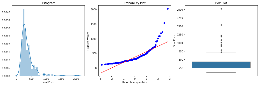
The first chart above hints at the following conclusions:
- Our target variable is not normally distributed, therefore we will carry out a log transformation.
- Our target variable is right-skewed.
- There are multiple outliers in the variable. Ordinary least squares regression might not be the optimal tool.
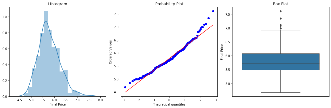
After carrying out the log transformation, we see that the distribution is more normal and there are fewer outliers.
Choosing predictors
#Get dummies for the categorical columns
df = pd.get_dummies(df, columns=['airport_distance', 'hotel_star_category'])
As a starting point, let us do a primitive selection of predictors based on correlation of the independent variables with the final price. Then we take the top five predictors, excluding the Number of Reviews, because we did not see any linear relationship between it and the final price.
# Price in SGD and Extra Fees dropped, since they make up "Final Price"
abs(df.drop(columns=['Price in SGD', 'Extra Fees']).corr())["Final Price"].sort_values(ascending = False)[1:]
hotel_star_category_five_star         0.701463
Guest Rating                          0.650943
hotel_star_category_low-class         0.563644
Number of Reviews                     0.259747
Distance from Changi Airport in km    0.252795
airport_distance_far                  0.193060
Love Hotel                            0.191550
airport_distance_middle               0.144981
Subway Access                         0.140708
hotel_star_category_four_star         0.038202
airport_distance_close                0.011188
Name: Final Price, dtype: float64
Let us choose four variables based on this correlation metric and the exploratory analysis performed before. The target will be a log-transformed version of the final price variable, in order to interpret the model coefficients as a percentage change and reduce the target skew.
After a couple of trial-and-error attempts of running the regression, the following predictors were chosen into the final model. The commented out code labels an example of variables which were tested but left out. The omitted predictors were left out either because they showed multicolinearity or they did not significantly increase the explanatory strength of the model.
df['Marina Bay'] = df['District'].apply(lambda x: 1 if x == 'Marina Bay' else 0)
df['Sentosa Island'] = df['District'].apply(lambda x: 1 if x == 'Sentosa Island' else 0)
independent_variables = df[[
    'Guest Rating',
   'hotel_star_category_low-class',
  #'Distance from Changi Airport in km',
    'hotel_star_category_five_star',
    #"Number of Reviews",
   # 'Marina Bay',
 #   'Sentosa Island',
    ]]
target_variable = np.log(df['Final Price'])
Regressions Diagnostics
Define a regression diagnostic helper - based on code from https://jeffmacaluso.github.io/. Minor modifications were required to make the code runnable.
def linear_regression_assumptions(features, label, feature_names=None):
    """
    Tests a linear regression on the model to see if assumptions are being met
    """
    from sklearn.linear_model import LinearRegression

    # Setting feature names to x1, x2, x3, etc. if they are not defined
    if feature_names is None:
        feature_names = ['X'+str(feature+1) for feature in range(features.shape[1])]

    print('Fitting linear regression')
    # Multi-threading if the dataset is a size where doing so is beneficial
    if features.shape[0] < 100000:
        model = LinearRegression(n_jobs=-1)
    else:
        model = LinearRegression()

    model.fit(features, label)

    # Returning linear regression R^2 and coefficients before performing diagnostics
    r2 = model.score(features, label)
    print()
    print('R^2:', r2, '\n')
    print('Coefficients')
    print('-------------------------------------')
    print('Intercept:', model.intercept_)

    for feature in range(len(model.coef_)):
        print('{0}: {1}'.format(feature_names[feature], model.coef_[feature]))

    print('\nPerforming linear regression assumption testing')

    # Creating predictions and calculating residuals for assumption tests
    predictions = model.predict(features)
    df_results = pd.DataFrame({'Actual': label, 'Predicted': predictions})
    df_results['Residuals'] = abs(df_results['Actual']) - abs(df_results['Predicted'])


    def linear_assumption():
        """
        Linearity: Assumes there is a linear relationship between the predictors and
                   the response variable. If not, either a polynomial term or another
                   algorithm should be used.
        """
        print('\n=======================================================================================')
        print('Assumption 1: Linear Relationship between the Target and the Features')

        print('Checking with a scatter plot of actual vs. predicted. Predictions should follow the diagonal line.')

        # Plotting the actual vs predicted values
        sns.lmplot(x='Actual', y='Predicted', data=df_results, fit_reg=False, size=7)

        # Plotting the diagonal line
        line_coords = np.arange(df_results['Actual'].min(), df_results['Actual'].max())
        plt.plot(line_coords, line_coords,  # X and y points
                 color='darkorange', linestyle='--')
        plt.title('Actual vs. Predicted')
        plt.show()
        print('If non-linearity is apparent, consider adding a polynomial term')


    def normal_errors_assumption(p_value_thresh=0.05):
        """
        Normality: Assumes that the error terms are normally distributed. If they are not,
        nonlinear transformations of variables may solve this.

        This assumption being violated primarily causes issues with the confidence intervals
        """
        from statsmodels.stats.diagnostic import normal_ad
        print('\n=======================================================================================')
        print('Assumption 2: The error terms are normally distributed')
        print()

        print('Using the Anderson-Darling test for normal distribution')

        # Performing the test on the residuals
        p_value = normal_ad(df_results['Residuals'])[1]
        print('p-value from the test - below 0.05 generally means non-normal:', p_value)

        # Reporting the normality of the residuals
        if p_value < p_value_thresh:
            print('Residuals are not normally distributed')
        else:
            print('Residuals are normally distributed')

        # Plotting the residuals distribution
        plt.subplots(figsize=(12, 6))
        plt.title('Distribution of Residuals')
        sns.distplot(df_results['Residuals'])
        plt.show()

        print()
        if p_value > p_value_thresh:
            print('Assumption satisfied')
        else:
            print('Assumption not satisfied')
            print()
            print('Confidence intervals will likely be affected')
            print('Try performing nonlinear transformations on variables')


    def multicollinearity_assumption():
        """
        Multicollinearity: Assumes that predictors are not correlated with each other. If there is
                           correlation among the predictors, then either remove prepdictors with high
                           Variance Inflation Factor (VIF) values or perform dimensionality reduction

                           This assumption being violated causes issues with interpretability of the
                           coefficients and the standard errors of the coefficients.
        """
        from statsmodels.stats.outliers_influence import variance_inflation_factor
        print('\n=======================================================================================')
        print('Assumption 3: Little to no multicollinearity among predictors')

        # Plotting the heatmap
        plt.figure(figsize = (10,8))
        sns.heatmap(features.corr(), annot=True)
        plt.title('Correlation of Variables')
        plt.show()

        print('Variance Inflation Factors (VIF)')
        print('> 10: An indication that multicollinearity may be present')
        print('> 100: Certain multicollinearity among the variables')
        print('-------------------------------------')

        # Gathering the VIF for each variable
        VIF = [variance_inflation_factor(features.values, i) for i in range(features.shape[1])]
        for idx, vif in enumerate(VIF):
            print('{0}: {1}'.format(features.columns[idx], vif))

        # Gathering and printing total cases of possible or definite multicollinearity
        possible_multicollinearity = sum([1 for vif in VIF if vif > 10])
        definite_multicollinearity = sum([1 for vif in VIF if vif > 100])
        print()
        print('{0} cases of possible multicollinearity'.format(possible_multicollinearity))
        print('{0} cases of definite multicollinearity'.format(definite_multicollinearity))
        print()

        if definite_multicollinearity == 0:
            if possible_multicollinearity == 0:
                print('Assumption satisfied')
            else:
                print('Assumption possibly satisfied')
                print()
                print('Coefficient interpretability may be problematic')
                print('Consider removing variables with a high Variance Inflation Factor (VIF)')
        else:
            print('Assumption not satisfied')
            print()
            print('Coefficient interpretability will be problematic')
            print('Consider removing variables with a high Variance Inflation Factor (VIF)')


    def autocorrelation_assumption():
        """
        Autocorrelation: Assumes that there is no autocorrelation in the residuals. If there is
                         autocorrelation, then there is a pattern that is not explained due to
                         the current value being dependent on the previous value.
                         This may be resolved by adding a lag variable of either the dependent
                         variable or some of the predictors.
        """
        from statsmodels.stats.stattools import durbin_watson
        print('\n=======================================================================================')
        print('Assumption 4: No Autocorrelation')
        print('\nPerforming Durbin-Watson Test')
        print('Values of 1.5 < d < 2.5 generally show that there is no autocorrelation in the data')
        print('0 to 2< is positive autocorrelation')
        print('>2 to 4 is negative autocorrelation')
        print('-------------------------------------')
        durbinWatson = durbin_watson(df_results['Residuals'])
        print('Durbin-Watson:', durbinWatson)
        if durbinWatson < 1.5:
            print('Signs of positive autocorrelation', '\n')
            print('Assumption not satisfied', '\n')
            print('Consider adding lag variables')
        elif durbinWatson > 2.5:
            print('Signs of negative autocorrelation', '\n')
            print('Assumption not satisfied', '\n')
            print('Consider adding lag variables')
        else:
            print('Little to no autocorrelation', '\n')
            print('Assumption satisfied')


    def homoscedasticity_assumption():
        """
        Homoscedasticity: Assumes that the errors exhibit constant variance
        """
        print('\n=======================================================================================')
        print('Assumption 5: Homoscedasticity of Error Terms')
        print('Residuals should have relative constant variance')

        # Plotting the residuals
        plt.subplots(figsize=(12, 6))
        ax = plt.subplot(111)  # To remove spines
        plt.scatter(x=df_results.index, y=df_results.Residuals, alpha=0.5)
        plt.plot(np.repeat(0, df_results.index.max()), color='darkorange', linestyle='--')
        ax.spines['right'].set_visible(False)  # Removing the right spine
        ax.spines['top'].set_visible(False)  # Removing the top spine
        plt.title('Residuals')
        plt.show()
        print('If heteroscedasticity is apparent, confidence intervals and predictions will be affected')


    linear_assumption()
    normal_errors_assumption()
    multicollinearity_assumption()
    autocorrelation_assumption()
    homoscedasticity_assumption()
linear_regression_assumptions(independent_variables, np.log(df['Final Price']))
Fitting linear regression

R^2: 0.7458869991458861

Coefficients
-------------------------------------
Intercept: 4.116529610144164
X1: 0.22041960962763665
X2: -0.24600661009310965
X3: 0.42793456641283856

Performing linear regression assumption testing

=======================================================================================
Assumption 1: Linear Relationship between the Target and the Features
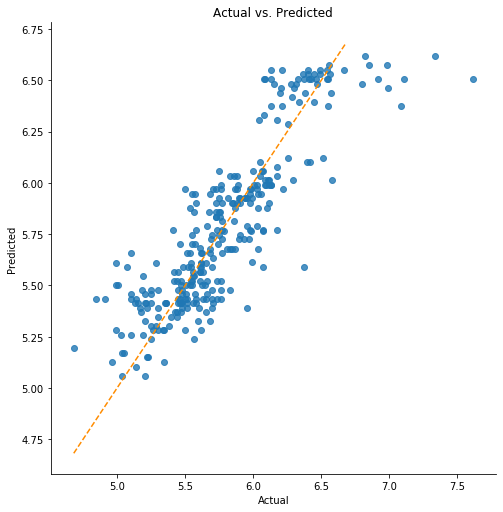
Checking with a scatter plot of actual vs. predicted. Predictions should follow the diagonal line.


/usr/local/lib/python3.6/dist-packages/seaborn/regression.py:574: UserWarning: The `size` parameter has been renamed to `height`; please update your code.
  warnings.warn(msg, UserWarning)
If non-linearity is apparent, consider adding a polynomial term

=======================================================================================
Assumption 2: The error terms are normally distributed

Using the Anderson-Darling test for normal distribution
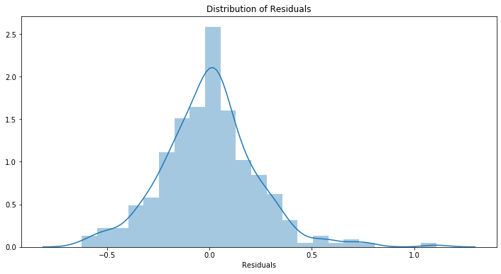
p-value from the test - below 0.05 generally means non-normal: 0.0003691235978455108
Residuals are not normally distributed
Assumption not satisfied

Confidence intervals will likely be affected
Try performing nonlinear transformations on variables

=======================================================================================
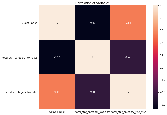
Assumption 3: Little to no multicollinearity among predictors
Variance Inflation Factors (VIF)
> 10: An indication that multicollinearity may be present
> 100: Certain multicollinearity among the variables
-------------------------------------
Guest Rating: 2.761822864159822
hotel_star_category_low-class: 2.167209737518528
hotel_star_category_five_star: 1.5946131266412962

0 cases of possible multicollinearity
0 cases of definite multicollinearity

Assumption satisfied

=======================================================================================
Assumption 4: No Autocorrelation

Performing Durbin-Watson Test
Values of 1.5 < d < 2.5 generally show that there is no autocorrelation in the data
0 to 2< is positive autocorrelation
>2 to 4 is negative autocorrelation
-------------------------------------
Durbin-Watson: 2.0454945834945004
Little to no autocorrelation

Assumption satisfied

=======================================================================================
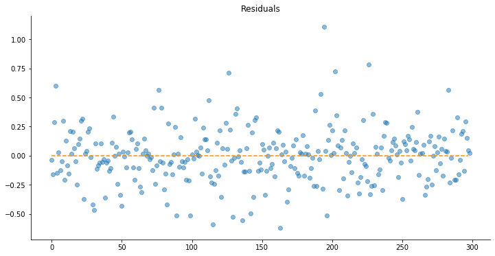
Assumption 5: Homoscedasticity of Error Terms
Residuals should have relative constant variance
If heteroscedasticity is apparent, confidence intervals and predictions will be affected
We see that:
1) The model somehow satisfies the linearity assumption, however, there are many outliers. It could be wort to try out robust regression, such as the Huber estimator.
2) The residuals are not normally distributed. That means that we should not rely much on our p-values and the model should not be used for inference. However, we might argue that since we are working with all hotels in Singapore, we have population data, not a sample. Therefore, we can take the coefficients as they are.
An opposing opinion would be that we are working with a sample, since we took only a snapshot at a point of time.
3) Multicolinearity seems to be not an issue here, based on the VIFs. In contrast, the correlation matrix shows a considerable correlation between the guest rating and the hotels starts.
Guest rating is an all-encompasing variable, which would benefit from decomposing it into specific factors.
4) The data seems to be homoskedastic, except for a few points, which are the already discussed outliers.
import statsmodels.api as sm


X = sm.add_constant(independent_variables) # adding a constant

model = sm.OLS(target_variable, X).fit()
predictions = model.predict(X)

print_model = model.summary()
print(print_model)
                            OLS Regression Results
==============================================================================
Dep. Variable:            Final Price   R-squared:                       0.746
Model:                            OLS   Adj. R-squared:                  0.743
Method:                 Least Squares   F-statistic:                     288.6
Date:                Sun, 16 Feb 2020   Prob (F-statistic):           2.07e-87
Time:                        22:19:34   Log-Likelihood:                 12.835
No. Observations:                 299   AIC:                            -17.67
Df Residuals:                     295   BIC:                            -2.869
Df Model:                           3
Covariance Type:            nonrobust
=================================================================================================
                                    coef    std err          t      P>|t|      [0.025      0.975]
-------------------------------------------------------------------------------------------------
const                             4.1165      0.186     22.087      0.000       3.750       4.483
Guest Rating                      0.2204      0.023      9.672      0.000       0.176       0.265
hotel_star_category_low-class    -0.2460      0.037     -6.703      0.000      -0.318      -0.174
hotel_star_category_five_star     0.4279      0.043      9.940      0.000       0.343       0.513
==============================================================================
Omnibus:                       30.388   Durbin-Watson:                   2.045
Prob(Omnibus):                  0.000   Jarque-Bera (JB):               68.120
Skew:                           0.507   Prob(JB):                     1.61e-15
Kurtosis:                       5.107   Cond. No.                         111.
==============================================================================

Warnings:
[1] Standard Errors assume that the covariance matrix of the errors is correctly specified.


/usr/local/lib/python3.6/dist-packages/numpy/core/fromnumeric.py:2495: FutureWarning: Method .ptp is deprecated and will be removed in a future version. Use numpy.ptp instead.
  return ptp(axis=axis, out=out, **kwargs)
After generating an output using statmodels, we see that the predictor with the highest coeffcient is the hotel’s belonging to the five-star category, which increases its price by 40%, ceteris paribus.
Second comes association with low-star hotels which decreases the price by around 24%.
The last predictor is the guest rating, where we see a 22% increase in price for every rating point.
Summary, Issues and next steps
We have created an extremely simple OLS regression with only three variables based on hotel stars and guest rating. When using it we should consider the following remarks:
1) The model is extremely simple - there are only three variables. We should collect more data, since we are very likely suffering from omitted variable bias. I assume that predictors such as investment into the building of the hotel, number of annual visitors, hotel capacity, etc. could improve the model.
2) The presence of outliers is influencing the regression coefficients. A remedy for this problem would be using robust regression or using predictors that would capture the reason why hotels like Marina Bay Sands stand out.
3) We could use interaction terms between the variables.
4) An interesting excercise would be to collect new data about the hotels today, and test whether our model is still acceptable.